Overpass API > Blog >
Published: 2018-07-16
In this concluding blog entry for the Overpass API version 0.7.55, the notion of derived geometries are introduced. This is the framework for feature requests that require to churn OSM elements: For example, simplifying a way is useful, but inevitably changes the member list of that way. Thus the object you get is quite different from the OSM object you asked for.
There are two substantially different use cases to churn OSM objects:
The first is to get insight where otherwise one gets lost in the sheer number of objects. As an example, an analysis of the tag operator on railways in Northrhine-Westphalia is developed in section Tag Distribution.
The other, more problematic yet useful use case is to auto-convert OSM data on the fly. The above mentioned per-object simplication is such a case. There are, always have been, and probably ever will be misguided people who try to "improve" the OSM database by doing auto-conversion as edits to the database. There are several problems with mechanical edits. For this reason, the design of Overpass API shall do its best to defeat such edits. In particular, any such conversion strips the version info to prevent you from accidentially uploading churned data.
However, this churn feature has its legit use case rather to counter the convenience argument of mechanical edits: Why should you alter the OSM database if you could get your processed data as convenient as with a source edit by converting it on the fly, even without needing a conversion chain? Please note that in most practical use cases for performance reasons you will be better off doing the conversion yourself. But the recommandation to use a script at the target has in the past muted not every discussion for a mechanical edit.
From this version on, you can as geometry compute and attach a GeoJSON geometry to any derived object. GeoJSON has its caveats as explained below, but at least it is relatively popular.
However, tyrasd has deemed GeoJSON directly from Overpass API as too complex for the moment being. But he has assured that he will revisit that decision if there is demand. Therefore, all examples are illustrated on a temporary instance (source code) of Overpass Turbo. I will try my best to ask Martin again. So, please give affirmative feedback to me or Martin if you want to get GeoJSON to Overpass Turbo.
We want to get a good understanding how values of a tag are distributed in a small region. In particular, we want to check whether the operator values of the railway network in the Ruhrgebiet make sense. The Ruhrgebiet has a huge connected light rail network operated by half a dozen or so different companies.
A simple check which values exist shows that of virtually every company there exist spelling variants or outdated names have survived: (Please remeber that you have to copy and paste at the moment to the temporary instance)
[out:csv(num,length,operator)];
area[name="Ruhrgebiet"];
way[railway][operator](area);
for (t["operator"])
{
  make stat operator=_.val,num=count(ways),length=sum(length());
  out;
}
Line 1 lets the result become a CSV file. Line 2 selects the Ruhrgebiet as area to search in and line 3 requests all ways that have both a key railway and a key operator in that area. The for statement in line 4 lets the subsequent block (lines 5 to 8) be executed once for every value that exists for t["operator"] in the found set.
Line 6 generates one aggregating object per loop execution: _.val is the value of this loop, count(ways) counts the number of ways that are in the set for this loop, and sum(...) aggregates per summing up numbers over what its argument evaluates to per object: here, length() returns the length per object in meters. These values are assigned to the tags operator, num, and length as indicated by the syntax.
Line 7 outputs per loop the generated object. The set tags from line 6 match for that purpose the tags requested as columns in line 1.
The most straightforward way to check what is going on is to return all involved elements:
area[name="Ruhrgebiet"];
way[railway][operator](area);
out geom;
Unfortunately, you see a well-filled map, but get no clue which of the elements has what value.
The is where the derived geometry can help. We can instead get exactly one point per value: (Copy & paste here)
area[name="Ruhrgebiet"];
way[railway][operator](area);
for (t["operator"])
{
  make stat operator=_.val,num=count(ways),length=sum(length()),
      ::geom=center(gcat(geom()));
  out geom;
}
The changes to the first request are: Keep with the default XML mode by omitting the first line. And in the make statement, we assign to a special value for setting geometry, ::geom. As opposed to the textual value, we need to assign a geometry to this key: The evaluator center(...) returns the center of the bounding box of whatever geometry it gets. We want to get the center of all the geometry of the involved objects combined. Thus, we need an aggregator, and gcat(...) is the aggregator that simply piles up all the geometry it gets from the objects it iterates over. Finally, geom() just returns per object its geometry.
This still does not tell us how the values are spatially distributed. While we had too much information before, we now have too little. Let's try a different thing.
The convex hull of whatever geometry is the polygon that just wraps all the objects inside. I.e., we get a glimpse about how disperse the objects are: (Copy & paste here)
area[name="Ruhrgebiet"];
way[railway][operator](area);
for (t["operator"])
{
  make stat operator=_.val,num=count(ways),length=sum(length()),
      ::geom=hull(gcat(geom()));
  out geom;
}
Relative to the previous query, this one has almost no changes. We just have exchanged center(...) for hull(...). Like center, the evaluator hull takes a geometry as argument. It then returns the convex hull of the given geometry.
The biggest nuisance is that the operator representing the German national railway results in a huge polygon - use the magnifying glass symbol to see the full polygons. In fact it are two because the division responsible for the stations, DB Station&Service AG gets in Germany usually one operator value and the division for keeping the tracks, DB Netz AG, a different one.
We want to get rid of them. The easiest way is to exclude them in the initial request: (Copy & paste here)
area[name="Ruhrgebiet"];
way[railway][operator][operator!~"^DB"](area);
for (t["operator"])
{
  make stat operator=_.val,num=count(ways),length=sum(length()),
      ::geom=hull(gcat(geom()));
  out geom;
}
We just have added in line 2 a regular expression criterion that operator shall not start with DB.
Finally, we could also get the exact geometry as one object per value. It is just of little use at the moment because Overpass Turbo does not support to highlight the full object:
area[name="Ruhrgebiet"];
way[railway][operator~"^BO",i](area);
for (t["operator"])
{
  make stat operator=_.val,num=count(ways),length=sum(length()),
      ::geom=trace(gcat(geom()));
  out geom;
}
We have exchanged hull(...) for trace(...). The trace of a geomtry is the deduplicated version, i.e., each segment appears at most once. Additionally, I have reduced the scope from all values for operator not starting with DB to only values for operator starting with BO no matter if uppercase or lowercase. This is because this final step is about spelling variants of the operator BOGESTRA only.
Of course, the well-known approach of MapCSS is still working. But you need to list all the values you want to visualize manually. Please fill in the missing values from the tabular result of the first query. Because it is so tedious I suggest the approaches with auto-generated geometry instead.
area[name="Ruhrgebiet"];
way[railway][operator~"^BO",i](area);
out geom;
{{style:
way[operator=BOGESTRA] { color: red; }
way[operator=bogestra] { color: gold; }
way[operator=Bochum-Gelsenkirchener Straßenbahnen AG] { color: purple; }
way[operator=] { color: TODO; }
}}
A future version of OVerpass Turbo is likely able to just apply a different colour to each object. That is the point where the evaluator trace because handy. But I am sorry, neither me nor somebody else has implemented that so far.
We can now auto-generate stop areas, i.e. draw clusters of public transport objects that have the same name: (Copy & paste here)
area[name="Dortmund"]->.a;
( node[public_transport](area.a);
  node[highway=bus_stop](area.a);
  way[public_transport](area.a);
  rel[public_transport=platform](area.a); );
for (t["name"])
{
  make stop_area
      name=_.val,
      source=set("{"+type()+" "+id()+"}"),
      ::geom=hull(gcat(geom()));
  out geom;
}
Line 1 picks Dortmund as the area of choice. We assign the found area to the named set a to ensure that we can use in parallel to the default set and thus multiple times. Lines 2 to 5 are query statements for various public transport objects, all with some tags and all queries restricted to the area stored in set a. Line 6 declares the loop to run over groups by the expression t["name"]. In line 8 to 11, one aggregate object per group is defined. We aggregate over all object identifiers, pretty printed as "{"+type()+" "+id()+"}". And we aggreate over the geomtry by chaining geom(), gcat(...), and hull(...) as explained in the previous section.
There is one problem left: We get one large polygon across the results for the dispersed objects that have no name. We fix it with a extra line: (Copy & paste here)
area[name="Dortmund"]->.a;
( node[public_transport](area.a);
  node[highway=bus_stop](area.a);
  way[public_transport](area.a);
  rel[public_transport=platform](area.a); );
nwr._(if:is_tag("name"));
for (t["name"])
{
  make stop_area
      name=_.val,
      source=set("{"+type()+" "+id()+"}"),
      ::geom=hull(gcat(geom()));
  out geom;
}
In this extra line, line 6, nwr lets pass all kinds of OSM objects. The criterion ._ turns the query into an act of filtering the previous result. And the criterion (if:...) employs the evaluator is_tag("name") to keep exactly those objects that have the name tag set.
You may wonder why we use as type stop_area instead just way. I generally do suggest to use types distinct from node, way, and relation for derived objects. In addition, it is not yet decided and subsequently not implemented in Overpass Turbo to auto-detect for these typ values if the object is in strict OSM format or the format of a derived object.
I had for a long time deliberately refrained from implementing GeoJSON. The reasons are still important problems, thus I will explain them here. Nobody shall claim he had not been warned.
In a nutshell, GeoJSON assumes that the world were flat.
Overpass API assumes that the world is a (regular) sphere. The sphere model is for measurements and striahgt lines slightly off reality, the flat world model is often even in the wrong order of magnitude. We will walk through examples for the problems.
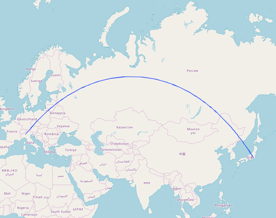
The first problem is that lines looking straight are not shortest connections (i.e. not the beeline) and that beelines do not look straight. Even worse, line segments that intersect in reality may give the impression of not intersecting and vice versa. The result is that the convex hulls introduced above need extra interpolation points. This can be some, but often are more than one expects. To illustrate the problem we build the beeline from Milano in Italy (IATA code BGY) to Tokyo in Japan (IATA code HND): (Copy & paste here)
[out:json];
( nwr["iata"="HND"];
  nwr["iata"="BGY"]; );
make beeline ::geom=hull(gcat(geom()));
out geom;
In line 1, JSON is chosen as the output format. This allows you to inspect the generated GeoJSON if you want to. Lines 2 and 3 collect every object tagged as the airport of Tokyo (HND) or Milano (BGY). In line 4, a single object with the convex hull of both airports combined is computed. In line 5, this object is printed.
The long edges of the polygon are in fact straight (up to rounding error). But the distortion of the flat world assumption lets them appear bent. In fact, the Overpass Turbo presentation uses a very common flat world model called Web Mercator that makes this problem slightly worse but it at least preserves angles. The flat world of GeoJSON does not even have that property.
For the intersection problem: The beeline does cross the borders of Latvija, but the phony-straight line does not.
The second problem is that the flat world assumption suggests both sides of the 180° line of longitude (called antimeridian) were the western resp. eastern end of the world. This has a couple of pitfalls, more and less obvious:
We compute the beeline from the airport of Tokyo (HND) to the airport of Los Angeles (LAX): (Copy & paste here)
[out:json];
( nwr["iata"="HND"];
  nwr["iata"="LAX"]; );
make beeline ::geom=hull(gcat(geom()));
out geom;
The antimeridian problem is the straight line from the eastern boundary to the western boundary. That line, of course, is not part of the flight plan but a presentation artifact. In fact, the GeoJSON specification does make precautions for the antimeridian and simply does not talk about line semgents crossing the antimeridian. But Leaflet apparently does assume the world ends at -180° longitude and 180° lonigtude. And it is likely that other consuming tool get this wonrg as well.
The third problem is that each of the poles is streched to a very long line. This is related to the problem that the distances close to the poles are the most distorted distances. But again, there are other problems. To illustrate this, we sketch the polar region as a polygon: (Copy & paste here)
[out:json];
make polar ::geom=poly(lstr(
    pt(66.5,0),
    pt(66.5,24),
    pt(66.5,48),
    pt(66.5,72),
    pt(66.5,96),
    pt(66.5,120),
    pt(66.5,144),
    pt(66.5,168),
    pt(66.5,-168),
    pt(66.5,-144),
    pt(66.5,-120),
    pt(66.5,-96),
    pt(66.5,-72),
    pt(66.5,-48),
    pt(66.5,-24)
    ));
out geom;
This is an example how to construct a derived geometry by hand: We ultimately want a polygon. Thus there is poly(...) that contains one or more linestring geometries, in this case one. This lstr(...) is made from multiple point geometries, all explicitly stated with pt(<Latitude>, <Longitude>).
This should have been a polygon that covers the north pole. Instead, it appears to cover only a strech of relatively small north-south-extent. It is not clear how you could enforce a polar polygon that in GeoJSON without knowing the limitations of the respective consuming software.
Finally, the adding of interpolation points is currently limited to polygons. For linestrings, the points are delivered verbatim. This may change infuture versions.
The rationale is that these linestring geometries are expected to be almost always OSM way geometries, and I deem it more important to verbatimly preserve that geometry than to compensate for consumer deficits. That linestrings are kept can been seenby the following example: (Copy & paste here)
[out:json];
make polar ::geom=lstr(
    pt(66.5,0),
    pt(66.5,120),
    pt(66.5,180),
    pt(66.5,-180),
    pt(66.5,-120)
    );
out geom;